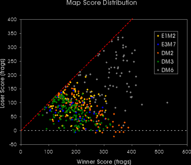
We can now compare all maps by adding all data of the previous graphs into one overview. The scores are now used as absolute values however.
DM6 clearly stands out with the highest scores. The rest of the results are crowded together, but the green DM3 scores are most compressed in the lower left, as could be expected from the average frag count already.
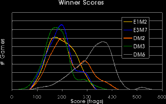
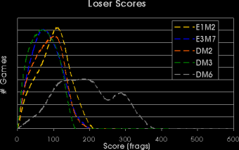
Instead of just plotting the raw scores, its interesting to make a histogram(1) or frequency distribution of them per map.
The DM6 curves stand out very clearly now. While the winning scores on that map are generally much higher then those anywhere else, its distribution of loser scores is very broad compared to that of all the other maps. The other loser score curves are rather symmetrical around their average value.
For E1M2 the winner score distribution is also rather broad, with any score between 150 and 250 occuring equally likely. The winner score distributions for E3M7, DM2 and DM3 have a more complex shape. On E3M7, DM2 and DM3, most of the rounds end with the winning team at a total of around 200 frags, but a in one third to one quarter of the rounds, the winners end with approximately 300 frags. DM2 and DM3 especially show two distinct humps.
Notes:
(1) A histogram is a curve often used in statistics. The height of the curve for any value of the horizontal axis is proportional to the amount of times it occured. To obtain a continues curve, occurances in a certain interval of the horizontal axis are considered together. Histograms are also referred to as 'frequency distributions'.